When teaching introductory linear regression, one of my favorite topics is “adjusted variable plots” or “added variable plots”. The basic idea is this: say you want to relate two sets of predictor variables, $\bf X$ and $\bf Z$, to a single response variable $\bf y$. One standard way to do this is through a multiple linear regression model, given in matrix/vector form by:

But let’s say that $\bf Z$ represents some control variables we definitely need to account for (e.g. age, sex), and we want to explore the nature of the relationship between $\bf X$ and $\bf y$, accounting for $\bf Z$. Or perhaps we want to fit a model relating $\bf y$ to just $\bf X$, controlling for $\bf Z$ by “regressing it out” beforehand. As it turns out, you can prove mathematically (see below) that if you regress out $\bf Z$ from both $\bf X$ and $\bf y$ then relate the adjusted $\bf y$ to the adjusted $\bf X$, you get the exact same estimate for β as in the multiple linear regression model stated above.

For the purpose of exploratory analysis, this is great news! We can simply:

1. Regress $\bf Z$ from $\bf X$ to produce $\bf \tilde{X}$,

2. Regress $\bf y$ from $\bf X$ to produce $\bf \tilde{y}$, then

3. Plot $\bf \tilde{y}$ versus $\bf \tilde{X}$ to get a visual impression of the relationship between $\bf y$ versus $\bf X$, while controlling for $\bf Z$.

A few things might be revealed:

• If $\bf X$ and $\bf Z$ are highly correlated, then after controlling for $\bf Z$ we might see that $\bf X$ does not add much. (Whereas if we naively plotted $\bf X$ against $\bf y$ without adjusting for $\bf Z$, the “marginal” relationship may appear strong, but this could just be driven by $\bf Z$.)

• We might see non-linear relationships between $\bf X$ and $\bf y$ more clearly, which we should account for in the model to avoid a misspecified model.

• We might see evidence of interactions between variables.

In any case, the ability to perform exploratory analysis between $\bf X$ and $\bf y$, while accounting for $\bf Z$, is pretty convenient.

Simulated Data Examples

Example 1

Here’s an example of this using simulated data. For simplicity, consider the case of a single variable X and single variable Z. In this example, both X and Z are correlated with the response variable Y. However, there is also strong correlation between X and Z. In this scenario, if we control for Z (“hold it constant”), the relationship between X and Y will be weaker than the marginal (“naive”) relationship between X and Y. Adjusted variable plots, such as those shown below, allow us to visually explore this relationship.

Generate simulated data:

#generate 3 independent variables X, Y, Z
set.seed(45873)
xyz0 <- matrix(rnorm(100*3), nrow=3, ncol=100)

#induce correlations between X, Y and Z
(cor_xyz <- matrix(c(1, 0.7, 0.85, 0.7, 1, 0.6, 0.85, 0.6, 1), nrow=3))

##      [,1] [,2] [,3]
## [1,] 1.00  0.7 0.85
## [2,] 0.70  1.0 0.60
## [3,] 0.85  0.6 1.00

cor_xyz_sqrt <- expm::sqrtm(cor_xyz)
xyz <- t(cor_xyz_sqrt %*% xyz0)
cor(xyz) #empirical correlation, should be close to cor_xyz

##           [,1]      [,2]      [,3]
## [1,] 1.0000000 0.6822354 0.8799130
## [2,] 0.6822354 1.0000000 0.6422735
## [3,] 0.8799130 0.6422735 1.0000000

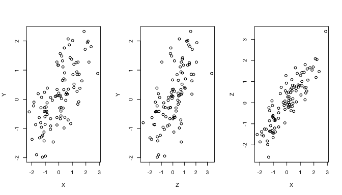
Plot the marginal relationships between the three variables:

#define X, Y, Z
X <- xyz[,1]
Y <- xyz[,2]
Z <- xyz[,3]

#plot marginal relationships
par(mfrow=c(1,3))
plot(X, Y)
plot(Z, Y)
plot(X, Z)

Plot the marginal vs. the adjusted relationship between X and Y:

#adjust both X and Y for Z, adding back in the mean
Y_adj <- residuals(lm(Y ~ Z)) + mean(Y)
X_adj <- residuals(lm(X ~ Z)) + mean(X)

library(ggplot2)
library(ggthemes)
library(gridExtra)
p1 <- qplot(X, Y) + geom_smooth(method='lm') + ggtitle('Marginal Relationship') + theme_few() + ylim(-2.5, 2.5)
p2 <- qplot(X_adj, Y_adj) + geom_smooth(method='lm') + ggtitle('Adjusted Relationship') + theme_few() + ylim(-2.5, 2.5)
grid.arrange(p1, p2, nrow=1)

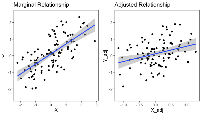
The main thing to notice is that the adjusted relationship is weaker than the marginal relationship between X and Y. In other words, if we only visualize the marginal relationship, we will get an overly optimistic picture of the relationship between X and Y (assuming we plan to include Z in the model). By contrast, the adjusted relationship plot adjusts for Z so we can get an accurate visual picture of the relationship between X and Y, accounting for Z.

Example 2

Another reason to use adjusted variable plots is to look for non-linear relationships between X and Y. If such non-linear relationships exist, we should build them into our model, hence avoiding a misspecified model. The existence and form of non-linear relationships can be difficult to see if we rely on marginal scatterplots. Here’s a simple simulated example where Y is related to X in a non-linear way:

#use the correlated x and z from above
#simulate y = beta0 + beta1*x^2 + gamma*z
beta0 <- 2
beta1 <- -2
gamma <- 5
Y <- beta0 + beta1*X^2 + gamma*Z + rnorm(100, mean = 0, sd = 0.1)

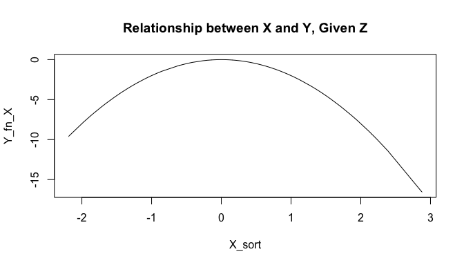
The true relationship between X and Y, for a fixed value of Z, is quadratic and looks like this:

X_sort <- sort(X)
Y_fn_X <- beta1*X_sort^2 
plot(X_sort, Y_fn_X, type='l', main='Relationship between X and Y, Given Z')

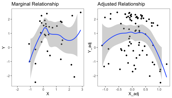
If we just visualize the marginal relationship between X and Y, this is not at all clear, as seen in the first plot below. The true quadratic relationship is much better revealed with the adjusted variable plot. Adjusting first for Z, we start to see the form of the relationship between X and Y more clearly. With this knowledge, we can incorporate non-linear terms in the model as appropriate.

#adjust both X and Y for Z, adding back in the mean
Y_adj <- residuals(lm(Y ~ Z)) + mean(Y)
X_adj <- residuals(lm(X ~ Z)) + mean(X)

p1 <- qplot(X, Y) + geom_smooth() + ggtitle('Marginal Relationship') + theme_few() + ylim(-2.5, 2.5)
p2 <- qplot(X_adj, Y_adj) + geom_smooth() + ggtitle('Adjusted Relationship') + theme_few() + ylim(-2.5, 2.5)
grid.arrange(p1, p2, nrow=1)

Proof of Adjusted Variables in OLS

We can show mathematically that if we first ``adjust’’ for a set of variables $\bf Z$, the marginal relationship between the adjusted versions of $\bf X$ and $\bf y$ is exactly the same as the relationship between the two when $\bf Z$ is included in the model. Let $\bf H$ denote the “hat matrix” when the design matrix is $\bf Z$, namely

Recall that $\bf H$ “puts the hat on” $\bf y$ when predicting $\bf y$ from $\bf Z$, i.e. $\bf\hat{y} = \bf Hy$. The residuals ${\bf\hat{y}} - {\bf y} = \bf (I-H)y$ are what we mean when we say “$\bf y$ adjusted for $\bf Z$”, which we are calling $\bf \tilde{y}$. So $\bf \tilde{y} = (I-H)y$, and $\bf \tilde{X} = (I-H)X$, where in both cases $\bf H$ is the hat matrix associated with design matrix $\bf Z$, given in the equation above.

Now that we have our adjusted variables $\bf \tilde{y}$ and $\bf \tilde{X}$, we can relate them through the model

The goal is to show that the OLS estimate for β in this model is exactly equal to the OLS estimate for β in the earlier model with $\bf X$ and $\bf Z$. First, let’s work out the OLS estimate for β in this model relating $\bf \tilde{y}$ to $\bf \tilde{X}$. We will use the fact that $\bf I - H$ is symmetric and idempotent, meaning that $\bf (I - H)(I - H) = (I - H)$.

$\tilde{\boldsymbol\beta} = ({\bf \tilde{X}’\tilde{X}})^{-1}{\bf \tilde{X}’\tilde{y}} = ({\bf X}’({\bf I - H}){\bf X})^{-1}{\bf X}’({\bf I - H}){\bf y}$

That was the easy part. :) Now let’s work out the OLS estimate for β in the earlier model relating $\bf y$ to $\bf X$ and $\bf Z$. Let $\bf W := \begin{bmatrix} \bf X & \bf Z \end{bmatrix}$

Since we are mainly interested in β, we need to work out the (1,1) and (1,2) blocks of $\bf A$, the inverse of the block matrix that appears above. Using standard formulas for block matrix inverses, we can obtain

$\hat{\boldsymbol\beta} = {\bf A_{11}X’y} + {\bf A_{12} Z’ y}$ $= ({\bf X}’{\bf X} - {\bf X}’{\bf Z}({\bf Z}’{\bf Z})^{-1}{\bf Z}’{\bf X})^{-1}{\bf X}’{\bf y} - ({\bf X}’{\bf X} - {\bf X}’{\bf Z}({\bf Z}’{\bf Z})^{-1}{\bf Z}’{\bf X})^{-1}{\bf X}’{\bf Z}({\bf Z}’{\bf Z})^{-1}{\bf Z}’{\bf y}$ $= ({\bf X}’{\bf X} - {\bf X}’{\bf H}{\bf X})^{-1}{\bf X}’{\bf y} - ({\bf X}’{\bf X} - {\bf X}’{\bf H}{\bf X})^{-1}{\bf X}’{\bf H}{\bf y}$ $= ({\bf X}’{\bf X} - {\bf X}’{\bf H}{\bf X})^{-1}({\bf X}’{\bf y} - {\bf X}’{\bf H}{\bf y})$ $= ({\bf X}({\bf I - H}){\bf X})^{-1}({\bf X}’({\bf I - H}){\bf y})$ $= ({\bf \tilde{X}}’{\bf \tilde{X}})^{-1}({\bf \tilde{X}}’{\bf \tilde{y}})$ $= \tilde{\boldsymbol\beta}$

Voila, it works!

Adjusted Variables in Penalized Regression

In many applications including my personal research, $\bf X$ is high-dimensional with the number of columns/variables p much greater than the number of rows/observations n. In this case, it’s common to use penalized regression techniques like ridge regression or LASSO. Does the theory behind adjusted variable plots hold up in this context?

If we fit a model relating a high-dimensional set of predictors $\bf X$ to $\bf y$ with either ridge or LASSO, the estimator for β is given by

where λ is a penalty parameter that is typically determined via cross-validation. If we also include confounders $\bf Z$ in the model, we can avoid including them in the penalization by setting λ = 0 for those variables. So our penalty matrix, rather than $\lambda \bf I$, becomes a block-diagonal matrix with $\lambda {\bf I}_p$ defining the upper-left block and zeros everywhere else.

As before, we can work out the estimate for β in the case of a penalty on $\bf X$. Letting $\bf W := \begin{bmatrix} \bf X & \bf Z \end{bmatrix}$ again, we can write:

Again we can use block matrix inverse formulas to obtain the estimator for β. Skipping some steps this time, we obtain

$\hat{\boldsymbol\beta}^R = \Big(({\bf X}’{\bf X} + \lambda{\bf I}) - {\bf X}’{\bf Z}({\bf Z}’{\bf Z})^{-1}{\bf Z}’{\bf X}\Big)^{-1}({\bf X}’{\bf y} - {\bf X}’{\bf Z}({\bf Z}’{\bf Z})^{-1}{\bf Z}’{\bf y})$ $= \Big(({\bf X}’{\bf X} + \lambda{\bf I}) - {\bf X}’{\bf H}{\bf X}\Big)^{-1}({\bf X}’{\bf y} - {\bf X}’{\bf H}{\bf y})$ $= \Big({\bf X}’{\bf X} - {\bf X}’{\bf H}{\bf X} + \lambda{\bf I}\Big)^{-1}({\bf X}’{\bf y} - {\bf X}’{\bf H}{\bf y})$ $= \Big({\bf X}’({\bf I - H}){\bf X} + \lambda{\bf I}\Big)^{-1}({\bf X}’({\bf I - H}){\bf y})$

$= \Big({\bf \tilde{X}}’{\bf \tilde{X}} + \lambda{\bf I}\Big)^{-1}({\bf \tilde{X}}’{\bf \tilde{y}})$

Success! The last line shows that the estimate for β in the model including $\bf Z$ is the same as what we would get if we related $\tilde{\bf y}$ ($\bf y$ adjusted for $\bf Z$) against $\tilde{\bf X}$ ($\bf X$ adjusted for $\bf Z$). Hence, the theory of adjusted variable plots in OLS holds for penalized regression methods like LASSO and ridge.

Take home message

When “adjusting for” confounding variables prior to fitting a model focusing only on the variables of interest, it is important to regress the confounders out from both $\bf X$ and $\bf y$. It is somewhat common to see $\bf Z$ only regressed from $\bf y$, disregarding the potential influence of $\bf Z$ on $\bf X$. This is a process known as “sequential processing” that can have unintended consequences.

In the case of prediction of $\bf y$ based on $\bf X$, failing to adjust $\bf X$ for $\bf Z$ as well can lead to attenuated prediction coefficients and ultimately worse prediction accuracy.

Whether you are using standard OLS or penalized regression in a high-dimensional setting, if you adjust both $\bf y$ and $\bf X$ for $\bf Z$, you can rest assured that it is fully equivalent to including $\bf Z$ as a confounder in your model.